Bayesian statistics

# Bayesian statistics
## Day 3
### Jason Lerch (with lots of slides from Chris Hammill)
### 2018/09/12

---

.medium {
  font-size: 80%;
}

.footnote {
  font-size: 75%;
  color: gray;
}

.smallcode {

}
.smallcode .remark-code {
  font-size: 50%
}

.smallercode {

}
.smallercode .remark-code {
  font-size: 75%
}

</style>

# Frequentist Null Hypothesis Testing

- To form conclusions in frequentism we typically lean on null hypothesis testing.
- Null hypotheses are parameter values for your model you'd like to disprove
- If your statistics (and more extreme statistics) would be very unlikely given your null model
  you reject the null hypothesis, and conclude that the null hypothesis is not correct.
- Choosing a threshold for this probability (e.g. 0.05) and rejecting when your p-value
  is below the threshold gives you a fixed probability of making a "Type I" error, 
  which conveniently is equal to your threshold.
- So if we reject all p-values when they are below 0.05 we have a 5% chance of
  rejecting when the null model is in fact true.
- If this is confusing, you're not alone, this is very hard to wrap your mind around.

---

# Fake data simulations

* Intepreting statistical models can be challenging
    
    * this is especially true in the presence of interactions
    
* It is much easier to understand what your statistical tests and models are doing if you know the ground truth.

* The easiest way to know the ground truth is to create it

* Let's do that here: 3 groups, 2 sexes, across age.

---

# Fake data simulations

```r
# create our age variable to range from 20 to 80
set.seed(1234) # this just makes sure we get same answer every time
age <- runif(120, min=20, max=80)
# set up the group and sex variables. Keep it balanced: 20 per group
group <- c(
  rep("G1", 40),
  rep("G2", 40),
  rep("G3", 40))
sex <- c(rep(rep(c("M", "F"), each=20), 3))
# Let's start simple, and assume that sex and group have no impact on
# our outcome, that there is a difference by sex at baseline, and
# that there is no difference by group at baseline
outcome_at_age20 <- 100
sex_diff_at_age_20 <- 3
change_per_year <- 0.5

outcome <- outcome_at_age20 + 
  ifelse(sex == "F", sex_diff_at_age_20, 0) + 
  (age-20)*change_per_year + 
  rnorm(length(age), mean=0, sd=2)

fake <- data.frame(age, sex, group, outcome)
```

---

# Fake data simulations

```r
suppressMessages(library(tidyverse))
fake %>% sample_n(18)
```

```
##          age sex group  outcome
## 1   26.82220   M    G1 104.7243
## 67  38.48569   F    G2 110.9800
## 55  29.17994   M    G2 104.6347
## 39  79.52903   F    G1 134.7103
## 97  38.01194   M    G3 108.5367
## 113 77.01830   F    G3 130.8438
## 76  51.15140   F    G2 117.8440
## 27  51.54185   F    G1 119.8709
## 92  74.02548   M    G3 127.2080
## 81  75.58403   M    G3 127.1239
## 108 27.79773   F    G3 106.7615
## 29  69.88070   F    G1 127.5572
## 95  26.31725   M    G3 103.4021
## 53  63.03630   M    G2 119.2986
## 33  38.28033   F    G1 115.5521
## 42  58.78437   M    G2 118.4427
## 79  39.23867   F    G2 114.4594
## 11  61.61548   M    G1 120.8215
```

---

# Fake data simulations

```r
theme_set(theme_minimal(18))
ggplot(fake) + aes(x=age, y=outcome, colour=group, shape=sex) +
  geom_point(size=3)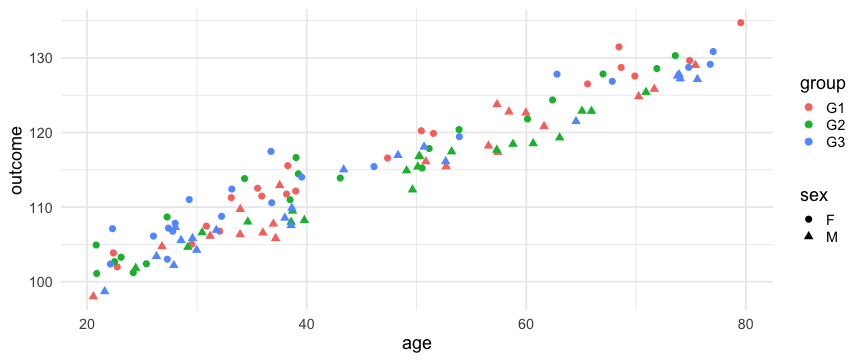 
```

![](bayes_files/figure-html/unnamed-chunk-3-1.png)

---

# Fake data simulations

```r
l1 <- lm(outcome ~ sex + group, fake)
summary(l1)
```

```
## 
## Call:
## lm(formula = outcome ~ sex + group, data = fake)
## 
## Residuals:
##      Min       1Q   Median       3Q      Max 
## -17.1449  -7.2691  -0.5505   6.0746  18.3803 
## 
## Coefficients:
##             Estimate Std. Error t value Pr(>|t|)    
## (Intercept)  116.330      1.634  71.190   <2e-16 ***
## sexM          -1.178      1.634  -0.721    0.473    
## groupG2       -1.595      2.001  -0.797    0.427    
## groupG3       -1.987      2.001  -0.993    0.323    
## ---
## Signif. codes:  0 '***' 0.001 '**' 0.01 '*' 0.05 '.' 0.1 ' ' 1
## 
## Residual standard error: 8.95 on 116 degrees of freedom
## Multiple R-squared:  0.01382,	Adjusted R-squared:  -0.01168 
## F-statistic: 0.5419 on 3 and 116 DF,  p-value: 0.6545
```

---

# Fake data simulations

```r
fake %>% mutate(l1 = predict(l1)) %>%
  ggplot() + aes(x=age, y=outcome, shape=sex, colour=group) +
  geom_point() + 
  geom_smooth(aes(y=l1), method="lm")
```

![](bayes_files/figure-html/unnamed-chunk-5-1.png)

---

# Fake data simulations

```r
l2 <- lm(outcome ~ age + sex + group, fake)
summary(l2)
```

```
## 
## Call:
## lm(formula = outcome ~ age + sex + group, data = fake)
## 
## Residuals:
##     Min      1Q  Median      3Q     Max 
## -3.9402 -1.1429 -0.1404  0.9960  5.7085 
## 
## Coefficients:
##               Estimate Std. Error t value Pr(>|t|)    
## (Intercept) 93.0544212  0.5867000 158.606  < 2e-16 ***
## age          0.5088154  0.0103152  49.327  < 2e-16 ***
## sexM        -2.9698983  0.3505404  -8.472 9.14e-14 ***
## groupG2     -0.6873279  0.4274064  -1.608    0.111    
## groupG3      0.0006102  0.4289073   0.001    0.999    
## ---
## Signif. codes:  0 '***' 0.001 '**' 0.01 '*' 0.05 '.' 0.1 ' ' 1
## 
## Residual standard error: 1.91 on 115 degrees of freedom
## Multiple R-squared:  0.9555,	Adjusted R-squared:  0.9539 
## F-statistic: 617.2 on 4 and 115 DF,  p-value: < 2.2e-16
```

---

# Fake data simulations

```r
fake %>% mutate(l2 = predict(l2)) %>%
  ggplot() + aes(x=age, y=outcome, shape=sex, 
                 colour=group, linetype=sex) +
  geom_point() + 
  geom_smooth(aes(y=l2), method="lm")
```

![](bayes_files/figure-html/unnamed-chunk-7-1.png)

---

# Fake data simulations

```r
l3 <- lm(outcome ~ age + sex, fake)
summary(l3)
```

```
## 
## Call:
## lm(formula = outcome ~ age + sex, data = fake)
## 
## Residuals:
##     Min      1Q  Median      3Q     Max 
## -3.9372 -1.2450 -0.3298  1.0972  5.9374 
## 
## Coefficients:
##             Estimate Std. Error t value Pr(>|t|)    
## (Intercept) 92.82950    0.51655  179.71  < 2e-16 ***
## age          0.50872    0.01033   49.23  < 2e-16 ***
## sexM        -2.96958    0.35270   -8.42 1.09e-13 ***
## ---
## Signif. codes:  0 '***' 0.001 '**' 0.01 '*' 0.05 '.' 0.1 ' ' 1
## 
## Residual standard error: 1.922 on 117 degrees of freedom
## Multiple R-squared:  0.9542,	Adjusted R-squared:  0.9534 
## F-statistic:  1218 on 2 and 117 DF,  p-value: < 2.2e-16
```

---

# Fake data simulations

```r
fake %>% mutate(l3 = predict(l3)) %>%
  ggplot() + aes(x=age, y=outcome, shape=sex, 
                 colour=group, linetype=sex) +
  geom_point() + 
  geom_smooth(aes(y=l3), method="lm")
```

![](bayes_files/figure-html/unnamed-chunk-9-1.png)

---

# Fake data simulations

```r
summary(lm(outcome ~ I(age-mean(age)) + sex, fake))
```

```
## 
## Call:
## lm(formula = outcome ~ I(age - mean(age)) + sex, data = fake)
## 
## Residuals:
##     Min      1Q  Median      3Q     Max 
## -3.9372 -1.2450 -0.3298  1.0972  5.9374 
## 
## Coefficients:
##                     Estimate Std. Error t value Pr(>|t|)    
## (Intercept)        116.03189    0.24873  466.49  < 2e-16 ***
## I(age - mean(age))   0.50872    0.01033   49.23  < 2e-16 ***
## sexM                -2.96958    0.35270   -8.42 1.09e-13 ***
## ---
## Signif. codes:  0 '***' 0.001 '**' 0.01 '*' 0.05 '.' 0.1 ' ' 1
## 
## Residual standard error: 1.922 on 117 degrees of freedom
## Multiple R-squared:  0.9542,	Adjusted R-squared:  0.9534 
## F-statistic:  1218 on 2 and 117 DF,  p-value: < 2.2e-16
```

---

# Fake data simulations

```r
l4 <- lm(outcome ~ age * sex * group, fake)
summary(l4)
```

```
## 
## Call:
## lm(formula = outcome ~ age * sex * group, data = fake)
## 
## Residuals:
##     Min      1Q  Median      3Q     Max 
## -4.4744 -1.2544 -0.2800  0.9125  5.5031 
## 
## Coefficients:
##                  Estimate Std. Error t value Pr(>|t|)    
## (Intercept)      91.39137    1.20782  75.667   <2e-16 ***
## age               0.54306    0.02418  22.463   <2e-16 ***
## sexM             -2.14636    1.84489  -1.163   0.2472    
## groupG2           0.57844    1.65397   0.350   0.7272    
## groupG3           3.14869    1.60859   1.957   0.0529 .  
## age:sexM         -0.01555    0.03659  -0.425   0.6717    
## age:groupG2      -0.02358    0.03451  -0.683   0.4958    
## age:groupG3      -0.06907    0.03331  -2.073   0.0405 *  
## sexM:groupG2      0.81197    2.73442   0.297   0.7671    
## sexM:groupG3     -2.08907    2.42185  -0.863   0.3903    
## age:sexM:groupG2 -0.02151    0.05507  -0.391   0.6969    
## age:sexM:groupG3  0.04528    0.04936   0.917   0.3610    
## ---
## Signif. codes:  0 '***' 0.001 '**' 0.01 '*' 0.05 '.' 0.1 ' ' 1
## 
## Residual standard error: 1.92 on 108 degrees of freedom
## Multiple R-squared:  0.9577,	Adjusted R-squared:  0.9534 
## F-statistic: 222.5 on 11 and 108 DF,  p-value: < 2.2e-16
```

---

# Fake data simulations

```r
fake %>% mutate(l4 = predict(l4)) %>%
  ggplot() + aes(x=age, y=outcome, shape=sex, 
                 colour=group, linetype=sex) +
  geom_point() + 
  geom_smooth(aes(y=l4), method="lm")
```

![](bayes_files/figure-html/unnamed-chunk-12-1.png)

---

# Interpreting these results

After fitting our models we're left with:

1. coefficient estimates
1. t-statistics
1. p-values

We know if our model assumptions are satisfied our t-statistics
  have a known distribution.

From this distribution we can figure out the probability of t-statistics
  as large or larger than the one we observed (p-value)

---

# Model comparions

```r
anova(l1, l2, l3, l4)
```

```
## Analysis of Variance Table
## 
## Model 1: outcome ~ sex + group
## Model 2: outcome ~ age + sex + group
## Model 3: outcome ~ age + sex
## Model 4: outcome ~ age * sex * group
##   Res.Df    RSS Df Sum of Sq         F Pr(>F)    
## 1    116 9292.4                                  
## 2    115  419.4  1    8873.0 2406.2571 <2e-16 ***
## 3    117  432.0 -2     -12.6    1.7097 0.1858    
## 4    108  398.2  9      33.7    1.0166 0.4315    
## ---
## Signif. codes:  0 '***' 0.001 '**' 0.01 '*' 0.05 '.' 0.1 ' ' 1
```

---
class: center

# And now for Bayesianism!

---
# Why Bayesian Statistics?

Have you ever...

1. Been confused about what a p-value means?
1. Been frustrated that a difference in significance doesn't mean a significant difference?
1. Known some values for a parameter are impossible but been unable to use that to your advantage?
1. Wanted to ask more interesting questions than whether or not a parameter is or isn't zero?
1. Wanted to use information from the literature to improve your estimates?

---

# Why Bayesian Statistics?

Have you ever...

Then Bayesian statistics might be right for you!

---

## How you ask?

1. **De-emphasize binary descisions.**
  Bayesians avoid null hypothesis tests, instead focusing on estimating their parameters of 
  interest, and reporting their uncertainty.
  
1. **Posterior Distributions**
  Bayesian analyses produce a distribution of possible parameter values (the posterior), that
  can be used to ask many interesting questions about values. E.g. what is the probability the
  effect in the hippocampus is larger than the effect in the anterior cingulate cortex.
  
1. **Prior Information**
  Bayesian analyses can use prior information. Bayesian analysis requires an *a priori* assessment
  of how likely certain parameters are. This can be vague (uninformative) or can precise (informative)
  and steer your analysis away from nonsensical results.

---

Reverend Thomas Bayes

![](images/Thomas_Bayes.gif)

---
class: middle

## Bayes' Theorem

- Bayes noticed this useful property for the probabilities for two events "A" and "B"

$$ \color{red}{P(A | B)} = \frac{{\color{blue}{P(B | A)}\color{orange}{P(A)}}}{\color{magenta}{P(B)}} $$

- `$\color{red}{P(A|B)}$`: The probability of A given that B happened
- `$\color{blue}{P(B|A)}$`: The probability of B given that A happened
- `$\color{orange}{P(A)}$`: The probability of A
- `$\color{magenta}{P(B)}$`: the probability of B

- Bayes did this in the context of the binomial distribution

---
class: middle
# But who's that behind him!

---
class: center

# It's Pierre-Simon Laplace

![](images/Pierre-Simon-Laplace.jpg)

---

## Bayesian Statistics

- Laplace generalized Bayes Theorem into it's modern form. While working on sex-ratios in French births.
- For light reading on the history of bayesianism consider reading [the theory that would not die](https://yalebooks.yale.edu/book/9780300188226/theory-would-not-die)

## Bayes in brief
- Start with some parameters `$\theta$`
- Collect some data `$D$`
- And deduce the probability of different values of `$\theta$` given that you observed `$D$`
- Key difference between Bayesianism and Frequentism is that view that `$\theta$` has an associated
  probability distribution. In frequentism `$\theta$` is an unknown constant.

---

# Different Probabilities

- Frequentists believe that probabilities represent the long-run proportion of events
- Under this model `$P(\theta)$` doesn't make much sense. 
- Ramsey and DeFinetti showed that probability can also represent degree of belief.
- Under this model `$P(\theta)$` is an assesment of what you think the the parameter will be.
- For some of the philosophy underpinning bayesian reasoning consider reading 
  [Bayesian philosophy of science](http://www.laeuferpaar.de/Papers/BookFrame_v1.pdf)
  
---
class: middle

# Bayes' Theorem Redux

$$ \color{red}{P(\theta | D)} = \frac{{\color{blue}{P(D | \theta)}\color{orange}{P(\theta)}}}{\color{magenta}{\int P(D | \theta)P(\theta)d\theta}} $$
**Posterior**: `$\color{red}{P(\theta|D)}$`:

the probability of our parameters given our data

**Likelihood**: `$\color{blue}{P(D|\theta)}$`

The probability of our data given our parameters

**Prior**: `$\color{orange}{P(\theta)}$`

The probability of our parameters before we saw the data

**Normalizing Constant**: `$\color{magenta}{\int P(D | \theta)P(\theta)d\theta}$`

The probability of the data averaged over all possible parameter sets

---

# Bayes' Theorem Redux

$$ \color{red}{P(\theta | D)} \propto \color{blue}{P(D | \theta)}\color{orange}{P(\theta)}$$

**Posterior**: `$\color{red}{P(\theta|D)}$`:

the probability of our parameters given our data

**Likelihood**: `$\color{blue}{P(D|\theta)}$`

The probability of our data given our parameters

**Prior**: `$\color{orange}{P(\theta)}$`

The probability of our parameters before we saw the data

---

# Bayes' Theorem Redux

$$ \color{red}{P(\theta | D)} \propto \color{orange}{P(\theta)}\color{blue}{P(D | \theta)}$$

**Posterior**: `$\color{red}{P(\theta|D)}$`:

the probability of our parameters given our data

**Prior**: `$\color{orange}{P(\theta)}$`

The probability of our parameters before we saw the data

**Likelihood**: `$\color{blue}{P(D|\theta)}$`

The probability of our data given our parameters

**Pardon the re-ordering**

---
class: middle

# Posterior

`$\color{red}{P(\theta|D)}$`

- The goal of bayesian statistics
- The posterior is probability distribution over parameters.
- Depends on the data we observed.
- Can be used to answer interesting questions. For
example how likely is an effect between two biologically meaninful boundaries.

---
class: middle

# Prior

`$\color{orange}{P(\theta)}$`

- This is what we knew before the experiment. 
- The prior is also a probability distribution over parameters.
- Doesn't depend on the data we saw.
- Gives a probability for any value the parameters could take.

---
class: middle

# Likelihood

`$\color{blue}{P(D | \theta)}$`

- This is how probable our data is given a hypothetical parameter set
- The likelihood is a probability distribution over data (not parameters)
- Is still a function of parameters.

---

# In words

$$ \color{red}{P(\theta | D)} \propto \color{orange}{P(\theta)}\color{blue}{P(D | \theta)}$$

The <font color="red">probability of parameters given our data</font> is proportional to <font color="orange">how probable we
thought they were before</font> adjusted by <font color="blue">how well they agree with the data we saw</font>.

![](images/posterior.gif)

---

# A first example

- Let's revisit linear modelling but this time from a bayesian stand-point.

$$ \textbf{y} = X\mathbf{\beta} + \mathbf{\epsilon} $$

We'll make our probabilistic views explicit

$$ \mathbf{\epsilon} \sim \mathbb{N}(0, \sigma) $$

`$\epsilon$` is normally distributed with some unknown variance `$\sigma$`

---

# Frequentist interpretation

- In frequentism `$\mathbf{\beta}$` is some fixed value.
- We can estimate standard errors for `$\beta$` and get p-values
  (likelihoods) that each component of `$\mathbf{\beta}$` is zero.
  
# Bayesian interpretation

- In bayesianism `$\mathbf{\beta}$` is a random variable that we're trying
  to learn about.
- In order to do this we have specify our prior belief about `$\mathbf{\beta}$`
- If we say we know nothing about `$\mathbf{\beta}$`, we get identical estimates
  to frequentism
- For our model we'll say `$\beta \sim \mathbb{N}(0,22.5)$`, the default.

---

# Fit a bayesian linear model

- For this we'll use the package `rstanarm`
-

```r
suppressMessages(library(rstanarm))
bl <- stan_glm(outcome ~ age + sex + group, data = fake)
```

```
## 
## SAMPLING FOR MODEL 'continuous' NOW (CHAIN 1).
## 
## Gradient evaluation took 0.000113 seconds
## 1000 transitions using 10 leapfrog steps per transition would take 1.13 seconds.
## Adjust your expectations accordingly!
## 
## 
## Iteration:    1 / 2000 [  0%]  (Warmup)
## Iteration:  200 / 2000 [ 10%]  (Warmup)
## Iteration:  400 / 2000 [ 20%]  (Warmup)
## Iteration:  600 / 2000 [ 30%]  (Warmup)
## Iteration:  800 / 2000 [ 40%]  (Warmup)
## Iteration: 1000 / 2000 [ 50%]  (Warmup)
## Iteration: 1001 / 2000 [ 50%]  (Sampling)
## Iteration: 1200 / 2000 [ 60%]  (Sampling)
## Iteration: 1400 / 2000 [ 70%]  (Sampling)
## Iteration: 1600 / 2000 [ 80%]  (Sampling)
## Iteration: 1800 / 2000 [ 90%]  (Sampling)
## Iteration: 2000 / 2000 [100%]  (Sampling)
## 
##  Elapsed Time: 0.100572 seconds (Warm-up)
##                0.075589 seconds (Sampling)
##                0.176161 seconds (Total)
## 
## 
## SAMPLING FOR MODEL 'continuous' NOW (CHAIN 2).
## 
## Gradient evaluation took 3.5e-05 seconds
## 1000 transitions using 10 leapfrog steps per transition would take 0.35 seconds.
## Adjust your expectations accordingly!
## 
## 
## Iteration:    1 / 2000 [  0%]  (Warmup)
## Iteration:  200 / 2000 [ 10%]  (Warmup)
## Iteration:  400 / 2000 [ 20%]  (Warmup)
## Iteration:  600 / 2000 [ 30%]  (Warmup)
## Iteration:  800 / 2000 [ 40%]  (Warmup)
## Iteration: 1000 / 2000 [ 50%]  (Warmup)
## Iteration: 1001 / 2000 [ 50%]  (Sampling)
## Iteration: 1200 / 2000 [ 60%]  (Sampling)
## Iteration: 1400 / 2000 [ 70%]  (Sampling)
## Iteration: 1600 / 2000 [ 80%]  (Sampling)
## Iteration: 1800 / 2000 [ 90%]  (Sampling)
## Iteration: 2000 / 2000 [100%]  (Sampling)
## 
##  Elapsed Time: 0.103304 seconds (Warm-up)
##                0.071193 seconds (Sampling)
##                0.174497 seconds (Total)
## 
## 
## SAMPLING FOR MODEL 'continuous' NOW (CHAIN 3).
## 
## Gradient evaluation took 1.4e-05 seconds
## 1000 transitions using 10 leapfrog steps per transition would take 0.14 seconds.
## Adjust your expectations accordingly!
## 
## 
## Iteration:    1 / 2000 [  0%]  (Warmup)
## Iteration:  200 / 2000 [ 10%]  (Warmup)
## Iteration:  400 / 2000 [ 20%]  (Warmup)
## Iteration:  600 / 2000 [ 30%]  (Warmup)
## Iteration:  800 / 2000 [ 40%]  (Warmup)
## Iteration: 1000 / 2000 [ 50%]  (Warmup)
## Iteration: 1001 / 2000 [ 50%]  (Sampling)
## Iteration: 1200 / 2000 [ 60%]  (Sampling)
## Iteration: 1400 / 2000 [ 70%]  (Sampling)
## Iteration: 1600 / 2000 [ 80%]  (Sampling)
## Iteration: 1800 / 2000 [ 90%]  (Sampling)
## Iteration: 2000 / 2000 [100%]  (Sampling)
## 
##  Elapsed Time: 0.124794 seconds (Warm-up)
##                0.076224 seconds (Sampling)
##                0.201018 seconds (Total)
## 
## 
## SAMPLING FOR MODEL 'continuous' NOW (CHAIN 4).
## 
## Gradient evaluation took 1.4e-05 seconds
## 1000 transitions using 10 leapfrog steps per transition would take 0.14 seconds.
## Adjust your expectations accordingly!
## 
## 
## Iteration:    1 / 2000 [  0%]  (Warmup)
## Iteration:  200 / 2000 [ 10%]  (Warmup)
## Iteration:  400 / 2000 [ 20%]  (Warmup)
## Iteration:  600 / 2000 [ 30%]  (Warmup)
## Iteration:  800 / 2000 [ 40%]  (Warmup)
## Iteration: 1000 / 2000 [ 50%]  (Warmup)
## Iteration: 1001 / 2000 [ 50%]  (Sampling)
## Iteration: 1200 / 2000 [ 60%]  (Sampling)
## Iteration: 1400 / 2000 [ 70%]  (Sampling)
## Iteration: 1600 / 2000 [ 80%]  (Sampling)
## Iteration: 1800 / 2000 [ 90%]  (Sampling)
## Iteration: 2000 / 2000 [100%]  (Sampling)
## 
##  Elapsed Time: 0.110427 seconds (Warm-up)
##                0.076907 seconds (Sampling)
##                0.187334 seconds (Total)
```

---

# How'd we do

```r
bl
```

```
## stan_glm
##  family:       gaussian [identity]
##  formula:      outcome ~ age + sex + group
##  observations: 120
##  predictors:   5
## ------
##             Median MAD_SD
## (Intercept) 93.0    0.6  
## age          0.5    0.0  
## sexM        -3.0    0.4  
## groupG2     -0.7    0.4  
## groupG3      0.0    0.4  
## sigma        1.9    0.1  
## 
## Sample avg. posterior predictive distribution of y:
##          Median MAD_SD
## mean_PPD 114.5    0.2 
## 
## ------
## For info on the priors used see help('prior_summary.stanreg').
```

---

# How does `lm` do?

```r
lmod <- lm(outcome ~ age + sex + group, fake)
summary(lmod)
```

---

# Side-By-Side

```r
coef(bl)
```

```
##  (Intercept)          age         sexM      groupG2      groupG3 
## 93.038424000  0.508874496 -2.965493553 -0.684045794  0.007676861
```

```r
coef(lmod)
```

```
##   (Intercept)           age          sexM       groupG2       groupG3 
## 93.0544212410  0.5088153748 -2.9698983483 -0.6873279028  0.0006101829
```

---

# Let's look at the posterior

```r
suppressPackageStartupMessages(library(bayesplot))
mcmc_areas(as.matrix(bl), pars=c("age"))
```

![](bayes_files/figure-html/unnamed-chunk-18-1.png)
---

# Let's look at the posterior

```r
mcmc_areas(as.matrix(bl), regex_pars = "sex|group")
```

![](bayes_files/figure-html/unnamed-chunk-19-1.png)

---

# What's happening here?

- `rstanarm` is creating a posterior for us, but how?
- in most bayesian textbooks this is shown first analytically for simple models.
  *this is not what stan does*
- Stan *approximates* the posterior using samples
- Samples are generated with markov-chain monte carlo (MCMC)
- For more details on the technique see Michael Betancourt's [A conceptual introduction to Hamiltonian Monte Carlo](https://arxiv.org/abs/1701.02434)

---

# The posterior revisited

```r
bl_post <- as.matrix(bl)

str(bl_post[,"age"])
```

```
##  num [1:4000] 0.504 0.5 0.516 0.511 0.518 ...
```

```r
summary(bl_post[,"age"])
```

```
##    Min. 1st Qu.  Median    Mean 3rd Qu.    Max. 
##  0.4738  0.5021  0.5089  0.5090  0.5158  0.5415
```

---

# What do we gain?

Intuitive use of probabilities:

What is the chance that the sex effect is greater than 0? Than 0.5?

```r
bl_post %>% as.data.frame %>%
  select(age) %>%
  summarize(gt0=mean(age>0),
            gt05=mean(age>0.5))
```

```
##   gt0    gt05
## 1   1 0.80525
```

---

# Priors

```r
prior_summary(bl)
```

```
## Priors for model 'bl' 
## ------
## Intercept (after predictors centered)
##  ~ normal(location = 0, scale = 10)
##      **adjusted scale = 88.98
## 
## Coefficients
##  ~ normal(location = [0,0,0,...], scale = [2.5,2.5,2.5,...])
##      **adjusted scale = [ 1.30,22.25,22.25,...]
## 
## Auxiliary (sigma)
##  ~ exponential(rate = 1)
##      **adjusted scale = 8.90 (adjusted rate = 1/adjusted scale)
## ------
## See help('prior_summary.stanreg') for more details
```

---

# Priors

```r
priors <- normal(0, c(2.5, 2.5, 0.5, 0.5), autoscale = F)
bl2 <- update(bl, prior=priors)
```

```
## 
## SAMPLING FOR MODEL 'continuous' NOW (CHAIN 1).
## 
## Gradient evaluation took 2.3e-05 seconds
## 1000 transitions using 10 leapfrog steps per transition would take 0.23 seconds.
## Adjust your expectations accordingly!
## 
## 
## Iteration:    1 / 2000 [  0%]  (Warmup)
## Iteration:  200 / 2000 [ 10%]  (Warmup)
## Iteration:  400 / 2000 [ 20%]  (Warmup)
## Iteration:  600 / 2000 [ 30%]  (Warmup)
## Iteration:  800 / 2000 [ 40%]  (Warmup)
## Iteration: 1000 / 2000 [ 50%]  (Warmup)
## Iteration: 1001 / 2000 [ 50%]  (Sampling)
## Iteration: 1200 / 2000 [ 60%]  (Sampling)
## Iteration: 1400 / 2000 [ 70%]  (Sampling)
## Iteration: 1600 / 2000 [ 80%]  (Sampling)
## Iteration: 1800 / 2000 [ 90%]  (Sampling)
## Iteration: 2000 / 2000 [100%]  (Sampling)
## 
##  Elapsed Time: 0.195112 seconds (Warm-up)
##                0.074192 seconds (Sampling)
##                0.269304 seconds (Total)
## 
## 
## SAMPLING FOR MODEL 'continuous' NOW (CHAIN 2).
## 
## Gradient evaluation took 1.5e-05 seconds
## 1000 transitions using 10 leapfrog steps per transition would take 0.15 seconds.
## Adjust your expectations accordingly!
## 
## 
## Iteration:    1 / 2000 [  0%]  (Warmup)
## Iteration:  200 / 2000 [ 10%]  (Warmup)
## Iteration:  400 / 2000 [ 20%]  (Warmup)
## Iteration:  600 / 2000 [ 30%]  (Warmup)
## Iteration:  800 / 2000 [ 40%]  (Warmup)
## Iteration: 1000 / 2000 [ 50%]  (Warmup)
## Iteration: 1001 / 2000 [ 50%]  (Sampling)
## Iteration: 1200 / 2000 [ 60%]  (Sampling)
## Iteration: 1400 / 2000 [ 70%]  (Sampling)
## Iteration: 1600 / 2000 [ 80%]  (Sampling)
## Iteration: 1800 / 2000 [ 90%]  (Sampling)
## Iteration: 2000 / 2000 [100%]  (Sampling)
## 
##  Elapsed Time: 0.236151 seconds (Warm-up)
##                0.0823 seconds (Sampling)
##                0.318451 seconds (Total)
## 
## 
## SAMPLING FOR MODEL 'continuous' NOW (CHAIN 3).
## 
## Gradient evaluation took 1.5e-05 seconds
## 1000 transitions using 10 leapfrog steps per transition would take 0.15 seconds.
## Adjust your expectations accordingly!
## 
## 
## Iteration:    1 / 2000 [  0%]  (Warmup)
## Iteration:  200 / 2000 [ 10%]  (Warmup)
## Iteration:  400 / 2000 [ 20%]  (Warmup)
## Iteration:  600 / 2000 [ 30%]  (Warmup)
## Iteration:  800 / 2000 [ 40%]  (Warmup)
## Iteration: 1000 / 2000 [ 50%]  (Warmup)
## Iteration: 1001 / 2000 [ 50%]  (Sampling)
## Iteration: 1200 / 2000 [ 60%]  (Sampling)
## Iteration: 1400 / 2000 [ 70%]  (Sampling)
## Iteration: 1600 / 2000 [ 80%]  (Sampling)
## Iteration: 1800 / 2000 [ 90%]  (Sampling)
## Iteration: 2000 / 2000 [100%]  (Sampling)
## 
##  Elapsed Time: 0.218637 seconds (Warm-up)
##                0.079457 seconds (Sampling)
##                0.298094 seconds (Total)
## 
## 
## SAMPLING FOR MODEL 'continuous' NOW (CHAIN 4).
## 
## Gradient evaluation took 1.4e-05 seconds
## 1000 transitions using 10 leapfrog steps per transition would take 0.14 seconds.
## Adjust your expectations accordingly!
## 
## 
## Iteration:    1 / 2000 [  0%]  (Warmup)
## Iteration:  200 / 2000 [ 10%]  (Warmup)
## Iteration:  400 / 2000 [ 20%]  (Warmup)
## Iteration:  600 / 2000 [ 30%]  (Warmup)
## Iteration:  800 / 2000 [ 40%]  (Warmup)
## Iteration: 1000 / 2000 [ 50%]  (Warmup)
## Iteration: 1001 / 2000 [ 50%]  (Sampling)
## Iteration: 1200 / 2000 [ 60%]  (Sampling)
## Iteration: 1400 / 2000 [ 70%]  (Sampling)
## Iteration: 1600 / 2000 [ 80%]  (Sampling)
## Iteration: 1800 / 2000 [ 90%]  (Sampling)
## Iteration: 2000 / 2000 [100%]  (Sampling)
## 
##  Elapsed Time: 0.287451 seconds (Warm-up)
##                0.091816 seconds (Sampling)
##                0.379267 seconds (Total)
```

---

# Priors and posteriors

```r
mcmc_areas(as.matrix(bl),  
 regex_pars = "sex|group")
```

![](bayes_files/figure-html/unnamed-chunk-24-1.png)
]
.pull-right[

```r
mcmc_areas(as.matrix(bl2), 
 regex_pars = "sex|group")
```

![](bayes_files/figure-html/unnamed-chunk-25-1.png)
]

---

# Priors and posteriors

![](bayes_files/figure-html/p1-1.png)

![](bayes_files/figure-html/p2-1.png)

---

# With real data now

Reload the data

```r
mice <- read_csv("mice.csv") %>%
  inner_join(read_csv("volumes.csv")) %>%
  mutate(Genotype = factor(Genotype, 
            levels=c("CREB +/+", "CREB +/-", "CREB -/-")),
         Condition=factor(Condition, levels=
      c("Standard", "Isolated Standard", "Exercise", "Enriched")))
```

```
## Parsed with column specification:
## cols(
##   Age = col_double(),
##   Sex = col_character(),
##   Condition = col_character(),
##   Mouse.Genotyping = col_character(),
##   ID = col_integer(),
##   Timepoint = col_character(),
##   Genotype = col_character(),
##   DaysOfEE = col_integer(),
##   DaysOfEE0 = col_integer()
## )
```

```
## Parsed with column specification:
## cols(
##   .default = col_double(),
##   ID = col_integer(),
##   Timepoint = col_character()
## )
```

```
## See spec(...) for full column specifications.
```

```
## Joining, by = c("ID", "Timepoint")
```

---

# Model at baseline

```r
b_base <- mice %>%
  filter(Timepoint == "Pre1") %>%
  stan_glm(hippocampus ~ Sex + Condition + Genotype, data=.)
```

```
## 
## SAMPLING FOR MODEL 'continuous' NOW (CHAIN 1).
## 
## Gradient evaluation took 4.7e-05 seconds
## 1000 transitions using 10 leapfrog steps per transition would take 0.47 seconds.
## Adjust your expectations accordingly!
## 
## 
## Iteration:    1 / 2000 [  0%]  (Warmup)
## Iteration:  200 / 2000 [ 10%]  (Warmup)
## Iteration:  400 / 2000 [ 20%]  (Warmup)
## Iteration:  600 / 2000 [ 30%]  (Warmup)
## Iteration:  800 / 2000 [ 40%]  (Warmup)
## Iteration: 1000 / 2000 [ 50%]  (Warmup)
## Iteration: 1001 / 2000 [ 50%]  (Sampling)
## Iteration: 1200 / 2000 [ 60%]  (Sampling)
## Iteration: 1400 / 2000 [ 70%]  (Sampling)
## Iteration: 1600 / 2000 [ 80%]  (Sampling)
## Iteration: 1800 / 2000 [ 90%]  (Sampling)
## Iteration: 2000 / 2000 [100%]  (Sampling)
## 
##  Elapsed Time: 0.168005 seconds (Warm-up)
##                0.16155 seconds (Sampling)
##                0.329555 seconds (Total)
## 
## 
## SAMPLING FOR MODEL 'continuous' NOW (CHAIN 2).
## 
## Gradient evaluation took 2.5e-05 seconds
## 1000 transitions using 10 leapfrog steps per transition would take 0.25 seconds.
## Adjust your expectations accordingly!
## 
## 
## Iteration:    1 / 2000 [  0%]  (Warmup)
## Iteration:  200 / 2000 [ 10%]  (Warmup)
## Iteration:  400 / 2000 [ 20%]  (Warmup)
## Iteration:  600 / 2000 [ 30%]  (Warmup)
## Iteration:  800 / 2000 [ 40%]  (Warmup)
## Iteration: 1000 / 2000 [ 50%]  (Warmup)
## Iteration: 1001 / 2000 [ 50%]  (Sampling)
## Iteration: 1200 / 2000 [ 60%]  (Sampling)
## Iteration: 1400 / 2000 [ 70%]  (Sampling)
## Iteration: 1600 / 2000 [ 80%]  (Sampling)
## Iteration: 1800 / 2000 [ 90%]  (Sampling)
## Iteration: 2000 / 2000 [100%]  (Sampling)
## 
##  Elapsed Time: 0.178642 seconds (Warm-up)
##                0.174038 seconds (Sampling)
##                0.35268 seconds (Total)
## 
## 
## SAMPLING FOR MODEL 'continuous' NOW (CHAIN 3).
## 
## Gradient evaluation took 3.2e-05 seconds
## 1000 transitions using 10 leapfrog steps per transition would take 0.32 seconds.
## Adjust your expectations accordingly!
## 
## 
## Iteration:    1 / 2000 [  0%]  (Warmup)
## Iteration:  200 / 2000 [ 10%]  (Warmup)
## Iteration:  400 / 2000 [ 20%]  (Warmup)
## Iteration:  600 / 2000 [ 30%]  (Warmup)
## Iteration:  800 / 2000 [ 40%]  (Warmup)
## Iteration: 1000 / 2000 [ 50%]  (Warmup)
## Iteration: 1001 / 2000 [ 50%]  (Sampling)
## Iteration: 1200 / 2000 [ 60%]  (Sampling)
## Iteration: 1400 / 2000 [ 70%]  (Sampling)
## Iteration: 1600 / 2000 [ 80%]  (Sampling)
## Iteration: 1800 / 2000 [ 90%]  (Sampling)
## Iteration: 2000 / 2000 [100%]  (Sampling)
## 
##  Elapsed Time: 0.195294 seconds (Warm-up)
##                0.146722 seconds (Sampling)
##                0.342016 seconds (Total)
## 
## 
## SAMPLING FOR MODEL 'continuous' NOW (CHAIN 4).
## 
## Gradient evaluation took 2.1e-05 seconds
## 1000 transitions using 10 leapfrog steps per transition would take 0.21 seconds.
## Adjust your expectations accordingly!
## 
## 
## Iteration:    1 / 2000 [  0%]  (Warmup)
## Iteration:  200 / 2000 [ 10%]  (Warmup)
## Iteration:  400 / 2000 [ 20%]  (Warmup)
## Iteration:  600 / 2000 [ 30%]  (Warmup)
## Iteration:  800 / 2000 [ 40%]  (Warmup)
## Iteration: 1000 / 2000 [ 50%]  (Warmup)
## Iteration: 1001 / 2000 [ 50%]  (Sampling)
## Iteration: 1200 / 2000 [ 60%]  (Sampling)
## Iteration: 1400 / 2000 [ 70%]  (Sampling)
## Iteration: 1600 / 2000 [ 80%]  (Sampling)
## Iteration: 1800 / 2000 [ 90%]  (Sampling)
## Iteration: 2000 / 2000 [100%]  (Sampling)
## 
##  Elapsed Time: 0.155294 seconds (Warm-up)
##                0.187006 seconds (Sampling)
##                0.3423 seconds (Total)
```

---
class: smallercode

# Model at baseline

```r
summary(b_base, digits=2)
```

```
## 
## Model Info:
## 
##  function:     stan_glm
##  family:       gaussian [identity]
##  formula:      hippocampus ~ Sex + Condition + Genotype
##  algorithm:    sampling
##  priors:       see help('prior_summary')
##  sample:       4000 (posterior sample size)
##  observations: 266
##  predictors:   7
## 
## Estimates:
##                              mean    sd      2.5%    25%     50%     75%  
## (Intercept)                  20.49    0.10   20.30   20.43   20.49   20.56
## SexM                          0.21    0.08    0.05    0.15    0.21    0.26
## ConditionIsolated Standard   -0.16    0.12   -0.40   -0.25   -0.17   -0.08
## ConditionExercise             0.03    0.11   -0.18   -0.04    0.03    0.11
## ConditionEnriched             0.14    0.10   -0.05    0.08    0.15    0.21
## GenotypeCREB +/-             -0.19    0.09   -0.37   -0.25   -0.19   -0.12
## GenotypeCREB -/-             -1.47    0.10   -1.66   -1.53   -1.47   -1.40
## sigma                         0.63    0.03    0.58    0.61    0.63    0.65
## mean_PPD                     20.13    0.06   20.02   20.09   20.13   20.17
## log-posterior              -268.26    2.10 -273.29 -269.38 -267.92 -266.76
##                              97.5%
## (Intercept)                  20.69
## SexM                          0.37
## ConditionIsolated Standard    0.08
## ConditionExercise             0.25
## ConditionEnriched             0.33
## GenotypeCREB +/-              0.00
## GenotypeCREB -/-             -1.28
## sigma                         0.69
## mean_PPD                     20.24
## log-posterior              -265.22
## 
## Diagnostics:
##                            mcse Rhat n_eff
## (Intercept)                0.00 1.00 3457 
## SexM                       0.00 1.00 4000 
## ConditionIsolated Standard 0.00 1.00 4000 
## ConditionExercise          0.00 1.00 4000 
## ConditionEnriched          0.00 1.00 4000 
## GenotypeCREB +/-           0.00 1.00 3419 
## GenotypeCREB -/-           0.00 1.00 4000 
## sigma                      0.00 1.00 4000 
## mean_PPD                   0.00 1.00 4000 
## log-posterior              0.05 1.00 1710 
## 
## For each parameter, mcse is Monte Carlo standard error, n_eff is a crude measure of effective sample size, and Rhat is the potential scale reduction factor on split chains (at convergence Rhat=1).
```

---

# Model at baseline

```r
mcmc_intervals(as.matrix(b_base), regex_pars = "Condition|Genotype|Sex")
```

![](bayes_files/figure-html/unnamed-chunk-29-1.png)

---

# Model at baseline

Is CREB +/- different from CREB -/-?

```r
b_base_post <- as.matrix(b_base)
colnames(b_base_post)
```

```
## [1] "(Intercept)"                "SexM"                      
## [3] "ConditionIsolated Standard" "ConditionExercise"         
## [5] "ConditionEnriched"          "GenotypeCREB +/-"          
## [7] "GenotypeCREB -/-"           "sigma"
```

```r
mean(b_base_post[,"GenotypeCREB +/-"] > b_base_post[,"GenotypeCREB -/-"])
```

```
## [1] 1
```

---

# Assignment (due Friday)

1. Compare accuracy of K-NN with logistic regression in predicting amygdala size on test dataset.

1. Split mice data into training, test, and validation. Optimize *K* hyperparameter
  of *K*-NN so the model has a higher performance in predicting amygdala size on test dataset. Report at least two different measures of binary classification on validation data. Use knn function in R.

1. Use random forest to predict genotype given volume of all regions in the brain. Optimize the number of trees in the random forest. Compare your training and validation accuracy, specificity, and sensitivity for each genotype (with a plot). Which variables have the highest feature importance (show in a plot)?

1. Generate a fake dataset with an interaction, and compute and compare linear model and bayesian linear model outputs.

1. Using whatever mix of bayesian, frequentist, or machine learning algorithms you like, conclude with a final statement about the effect of Genotype, Condition, and Time on hippocampal volume.

]