class: center, middle, inverse, title-slide # Logistic Regression ### Mehran Karimzadeh ### September 12, 2018 --- <style> .small { font-size: 65%; } .medium { font-size: 80%; } .smallcode { } .smallcode .remark-code { font-size: 50% } </style> ## Data and packages for these slides: ```r knitr::opts_chunk$set(echo = FALSE) # required_packages = c("caret", "tree", "randomForest", # "cowplot", "e1071") # install.packages(required_packages) require(tidyverse) require(cowplot) mice_df = read_csv("mice.csv") volume_df = read_csv("volumes.csv") mice = inner_join(mice_df, volume_df) ``` --- # Logistic regression --- ## Binary variables Can we predict gender given striatum volume? ```r mice$amygdala.group = ifelse(mice$amygdala > 10, 1, 0) ggplot(mice, aes(x=amygdala.group, y=striatum, group=amygdala.group)) + geom_boxplot() + theme_bw(base_size=18) ``` 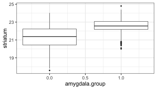<!-- --> --- ## Linear model for binary variables? * If the independent variable is binary, can we fit the linear model? ```r ggplot(mice, aes(x=striatum, y=amygdala.group)) + geom_point() + xlab("Volume of striatum") + ylab("Amygdala group") + geom_smooth(method="lm") + ggtitle("Amygdala group ~ Striatum volume") ``` 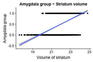<!-- --> --- ## Why we can't use linear model for classification? * Suppose we want to predict seizure, stroke, or overdose given some measurements from patients -- * If we model them as 1, 2, and 3 respectively, we are assuming order -- * Even in case of binary variables, our estimates may exceed range of [0, 1], making the interpretation unnecessarily hard -- * Any other reasons that contradict assumptions of the linear model? -- * Read this [blogpost](http://thestatsgeek.com/2015/01/17/why-shouldnt-i-use-linear-regression-if-my-outcome-is-binary) --- ## Logistic function * `\(\frac{L}{1 + e^{-k*(x - \sigma_0)}}\)` ```r logistic_function = function(input, curve_max=1, curve_steepness=1, sig_mid=0){ output = curve_max / (1 + exp(-curve_steepness * (input - sig_mid))) } input_vals = rnorm(50, sd=3) out_df = data.frame( X=input_vals, Y=logistic_function(input_vals)) ggplot(out_df, aes(x=X, y=Y)) + geom_line() ``` 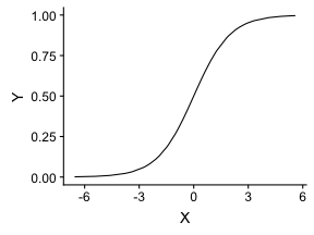<!-- --> --- ## Linear model for binary variables? 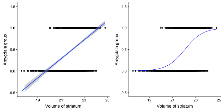<!-- --> --- ## Solving the logistic model * `\(p(X) = \beta_0\)` + `\(\beta X\)` -- * `\(p(X) = \frac{1}{1 + e^{\beta_0 + \beta X}} \rightarrow\)` estimating probability with logistic function -- * `\(\frac{p(X)}{1 - p(X)} = e^{\beta_0 + \beta X} \rightarrow\)` odds -- * `\(\text{log}(\frac{p(X)}{1 - p(X)}) = \beta_0 + \beta X \rightarrow\)` logit or log of odds -- * In linear model, `\(\beta\)` shows how a unit increase in *X* changes *Y* -- * The effect size `\(\beta\)` shows how a unit increase in *X* changes log odds -- * In linear regression, we used least squared to minimize mean squared error -- * In logistic regression, we use __maximum likelihood__ -- * `\(l(\beta_0, \beta) = \Pi_{i:y_i=1} p(x_i) \Pi_{i\prime:y_{i\prime}=0} (1 - p(x_{i\prime})) \rightarrow\)` Likelihood function --- # K-nearest neighbours * Example of a non-parametric, simple, and powerful machine learning method --- ## K-NN * Given a positive integer *K* and a datapoint `\(x_0\)`, identifies *K* points in training data which are closest to a datapoint `\(x_0\)`. -- * It then estimates the conditional probability for label of `\(x_0\)` given responses for its `\(K\)` nearest neighbours -- * Let's implement it in R! --- ## K-NN algorithm * Split data to training and test -- ```r split_ratio = 0.8 idx_train = sample(1:nrow(mice), size=floor(nrow(mice) * split_ratio)) train_df = mice[idx_train, ] test_df = mice[-idx_train, ] ``` --- * Predict amygdala size given volume of striatum and midbrain -- * Finding nearest neighbours ```r get_neighbours = function(test_data, train_df, K=5){ merged_df = rbind(test_data, train_df) dist_df = as.matrix(dist(merged_df, method="euclidean")) distances = as.numeric(dist_df[1, ]) idx_out = order(distances, decreasing=FALSE)[2:(K + 1)] ## Deduct 1 so the indices map to train_df instead of merged_df idx_out = idx_out - 1 return(idx_out) } ``` --- ## K-NN prediction ```r predictive_features = c("striatum", "midbrain") response = "amygdala.group" test_df$Posterior = NA for(i in 1:nrow(test_df)){ idx_neighbours = get_neighbours( test_df[i, predictive_features], train_df[, predictive_features]) labels = unlist(train_df[idx_neighbours, response]) prob = mean(labels) test_df$Posterior[i] = prob } ``` --- ## Calculating threshold-based metrics ```r suppressMessages(require(caret)) suppressMessages(require(e1071)) confMat = confusionMatrix( factor(test_df$Posterior > 0.5), factor(test_df$amygdala.group == 1)) print(as.data.frame(confMat$byClass)) ``` ``` ## confMat$byClass ## Sensitivity 0.8432836 ## Specificity 0.8000000 ## Pos Pred Value 0.7957746 ## Neg Pred Value 0.8467153 ## Precision 0.7957746 ## Recall 0.8432836 ## F1 0.8188406 ## Prevalence 0.4802867 ## Detection Rate 0.4050179 ## Detection Prevalence 0.5089606 ## Balanced Accuracy 0.8216418 ``` ```r print(paste("Accuracy =", signif(confMat$overall["Accuracy"], 3))) ``` ``` ## [1] "Accuracy = 0.821" ``` --- ## Plotting performance ```r train_df$Posterior = NA train_df$Dataset = "Training" test_df$Dataset = "Test" merged_df = rbind(train_df, test_df) ggplot(merged_df) + aes(x=striatum, y=midbrain, colour=Posterior > 0.5) + geom_point(alpha=0.5) + geom_point(data=test_df, aes(colour=Posterior > 0.5)) + theme_bw(base_size=16) + facet_grid(factor(amygdala.group)~Dataset) ``` 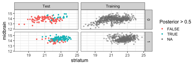<!-- --> -- --- # Random forest, in simple terms * Random forests can regress or classify, and they are made of hundreds of trees -- * Each tree uses some of data (samples) and some of the features -- * We identify which feature can classify (or regress) the outcome better -- * We split the data at the point which classifies training data best, and repeat the last step on each split until all data points are grouped -- * We build hundreds of trees based on training data. When it comes to new data, we use the majority vote to decide on the response for output variable --- ## Classification tree ```r require(tree) ``` ``` ## Loading required package: tree ``` ```r volume_df = read.csv("volumes.csv") volume_df = volume_df[, !colnames(volume_df) %in% c("ID", "Timepoint")] volume_df$amygdala.group = ifelse(volume_df$amygdala > 10, 1, 0) train_df = volume_df[idx_train, ] test_df = volume_df[-idx_train, ] tree_model = tree(factor(amygdala.group) ~.-amygdala, train_df) # summary(tree_model) ``` --- ## ```r pred_tree = predict(tree_model, test_df, type="class") confMat = confusionMatrix(pred_tree, factor(test_df$amygdala.group)) acc_tree = signif(confMat$overall["Accuracy"], 3) print(paste("Accuracy =", acc_tree)) ``` ``` ## [1] "Accuracy = 0.853" ``` ```r plot(tree_model) ``` 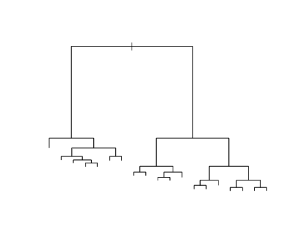<!-- --> ```r # text(tree_model, pretty=0) ``` --- ## Fitting a random forest ```r suppressMessages(require(randomForest)) rf_model = randomForest(factor(amygdala.group) ~.-amygdala, data=train_df, ntree=100, importance=TRUE) pred_rf = predict(rf_model, newdata=test_df) confMat = confusionMatrix(pred_rf, factor(test_df$amygdala.group)) acc_rf = signif(confMat$overall["Accuracy"], 3) print(paste("Accuracy RF =", acc_rf, "and tree =", acc_tree)) ``` ``` ## [1] "Accuracy RF = 0.892 and tree = 0.853" ``` --- ## Feature importance by random forest * Mean decrease Gini is the sum of Gini impurity of a feature across all trees. -- * Gini impurity is a measure of how often a randomly chosen element from the set would be incorrectly labeled ```r imp_df = as.data.frame(importance(rf_model)) imp_df$Feature = rownames(imp_df) imp_df = imp_df[ order(imp_df$MeanDecreaseGini, decreasing=TRUE)[1:10], ] imp_df$Feature = factor( imp_df$Feature, levels=imp_df$Feature[order(imp_df$MeanDecreaseGini)]) ``` --- ```r ggplot(imp_df) + aes(x=Feature, y=MeanDecreaseGini) + geom_bar(stat="identity", fill="purple") + coord_flip() ``` 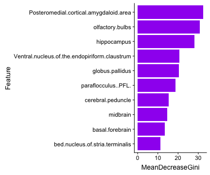<!-- --> --- # Assignment <!--1. Compare accuracy of K-NN with logistic regression in predicting amygdala size on test dataset. 2. Split mice data into training, test, and validation. Optimize *K* hyperparameter of *K*-NN so the model has a higher performance in predicting amygdala size on test dataset. Report at least two different measures of binary classification on validation data. Use knn function in R. 3. Use random forest to predict genotype given volume of all regions in the brain. Optimize the number of trees in the random forest. Compare your training and validation accuracy, specificity, and sensitivity for each genotype (with a plot). Which variables have the highest feature importance (show in a plot)? 4. Why do we split data into training, test, and validation? -->