```{r setup, include=FALSE} options(htmltools.dir.version = FALSE) ``` # Hello World The three challenges of statistical inference are¹: .footnote[ [1] From Andrew Gelman ] -- 1. Generalizing from sample to population -- 2. Generalizing from control to treatment group -- 3. Generalizing from observed measurements to underlying constructs of interest --- # Three laws of statistics .pull-left[ Arthur C. Clarke's three laws¹: 1. When a distinguished but elderly scientist states that something is possible, he is almost certainly right. When he states that something is impossible, he is very probably wrong. 1. The only way of discovering the limits of the possible is to venture a little way past them into the impossible. 1. Any sufficiently advanced technology is indistinguishable from magic. ] -- .pull-right[ Andrew Gelman's updates²: 1. When a distinguished but elderly scientist states that “You have no choice but to accept that the major conclusions of these studies are true,” don’t believe him. 2. The only way of discovering the limits of the reasonable is to venture a little way past them into the unreasonable. 3. Any sufficiently crappy research is indistinguishable from fraud. ] -- .small[ [1] https://en.wikipedia.org/wiki/Clarke%27s_three_laws [2] http://andrewgelman.com/2016/06/20/clarkes-law-of-research/ ] --- # The MBP statistics bootcamp Goals of this week: 1. Teach the theory and practice of statistics 1. Applied data analysis problem solving using R 1. Think hard about truth and replicability in science Slides, recommended readings, and extra resources here: https://jasonlerch.github.io/MBP-stats-2019/ (Will try and have slides for each day up the night before) --- # The MBP statistics bootcamp ```{r, echo=F} suppressMessages({ library(huxtable) library(tidyverse) }) ht <- tribble_hux( ~ Hour, ~ Monday, ~ Tuesday, ~ Wednesday, ~ Thursday, ~ Friday, "9-12", NA, NA, NA, NA, NA, "12-3", NA, NA, NA, NA, NA, # "1-3", NA, NA, NA, NA, NA, # "3-4", NA, NA, NA, NA, NA, add_colnames = TRUE ) %>% set_left_padding(10) %>% set_right_padding(10) bottom_border(ht)[1,] <- 1 right_border(ht)[,1] <- 1 ht[2,2] <- "Introduction. Data organization, descriptive statistics, plotting, basic models. " ht[3,2] <- "Group assignment #1" #rowspan(ht)[2, 2] <- 2 ht[2,3] <- "Probability in all its glory. Multiple linear models, interactions, p values. " ht[3,3] <- "Group assignment #2" #rowspan(ht)[2,3] <- 2 ht[2,4] <- "Hypothesis testing, searching for truth, multiple comparisons, and the crisis of replicability" #rowspan(ht)[4,4] <- 2 ht[3,4] <- "Group assignment #3" ht[2,5] <- "Putting it all together – analyzing a biomedical dataset from beginning to end. Review" #rowspan(ht)[4,5] <- 2 ht[3,5] <- "Group assignment #4" ht[2,6] <- "Presentations, exam" wrap(ht) <- TRUE escape_contents(ht) <- FALSE theme_basic(ht) ``` --- # Grading Exams (concepts only, no R): ```{r, echo=F} ht <- tribble_hux( ~ "What", ~ "When", ~ "How much", "Short exam", "Tuesday", "5%", "Short exam", "Wednesday", "5%", "Short exam", "Thursday", "5%", "Final exam", "Friday", "35%", add_colnames = TRUE) theme_basic(ht) ``` Group assignments and presentations (R analyses and concepts): ```{r, echo=F} ht <- tribble_hux( ~ "What", ~ "Due when", ~ "How much", "Group assignment #1", "Tuesday", "10%", "Group assignment #2", "Wednesday", "10%", "Group assignment #3", "Thursday", "10%", "Group assignment #4", "Friday", "10%", "Final presentation", "Friday", "10%", add_colnames = TRUE) theme_basic(ht) ``` --- # Exams * true/false, multiple choice, and short paragraphs. * each class begins with ~ 10 minute, short exam covering previous day. * final exam 30-60 minutes. -- .pull-left[ Sample questions: _Describe the null hypothesis_ _Identify elements of a box and whiskers plot (on a drawing)_ _Discuss analysis pre-registration advantages and disadvantages_ _TRUE/FALSE: if you compute a 95% confidence interval, you have a 95% chance of it containing the true value_ ] .pull-right[ ```{r, echo=FALSE} ggplot(data.frame(sample=rnorm(10000))) + aes(y=sample) + geom_boxplot() + xlab("") + ylab("") + scale_x_continuous(breaks = NULL) + scale_y_continuous(breaks = NULL) + theme_classic() ``` ] --- # Group assignments * split into small groups of 3-4. * we will assign groups. * will try to mix groups by R and programming expertise. * each group will be graded as a unit. * final presentation given by a member of the group with least R/programming expertise. --- class: inverse, center, middle # Let's get started --- # Statistical software .pull-left[ Common software 1. Excel 1. SPSS 1. SAS 1. matlab 1. python 1. R ] -- .pull-right[ Ups and downs of R 1. Open source, free, and powerful. 1. If a statistical test exists, it likely exists in R. 1. Literate programming/self documenting analyses. 1. Very strong in bioinformatics. 1. Steeper learning curve. 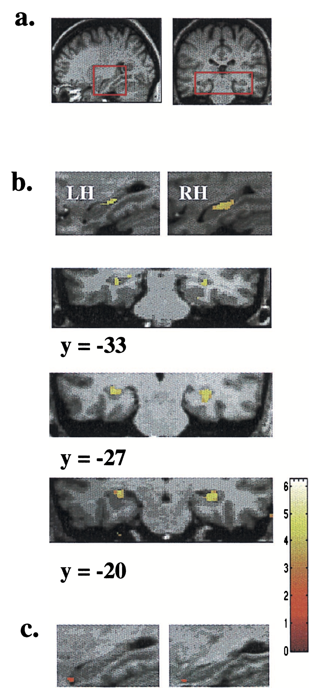] --- class: inverse, middle, center # Reading and summarizing our data --- # Intro to our dataset .pull-left[ How do our brains change as we learn or undergo new experiences? Earliest evidence that our brains are _plastic_ at larger, or _mesoscopic_, scales came from a study of taxi drivers in London, UK. Mechanism of how that happens is unclear. 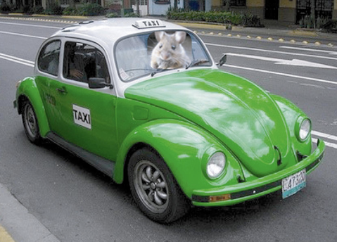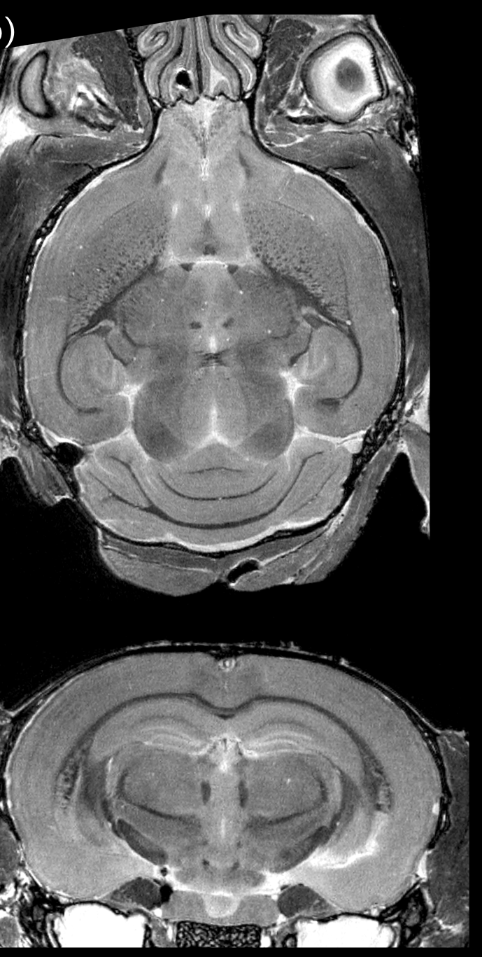] .pull-right[ ] .footnote[PhD Thesis of Dulcie Vousden] --- # Mouse models .pull-left[ We can create taxi driving mice. Use high-field MRI to get similar readout as in humans. Use genetic models to test hypotheses of implicated pathways. Use RNA sequencing to assess what changes per genotype or experimental group. ] .pull-right[ ] --- # The dataset ```{r, include=FALSE} #mice <- readRDS("mice.Rds") mice <- read.csv("mice.csv") volumes <- read.csv("volumes.csv", check.names = F) mice <- mice %>% inner_join(volumes) ``` -- There are `r length(unique(mice$ID))` mice in this dataset, with MRI scans acquired at `r length(unique(mice$Timepoint))` timepoints. -- We have 3 genotypes: `r levels(mice$Genotype)` -- There are 4 environmental conditions: `r levels(mice$Condition)` -- MRIs were acquired at every timepoint, and the brains automatically segmented into `r ncol(mice$vols_combined)` regions. -- There are good reasons to believe that the hippocampus and the dentate gyrus of the hippocampus will be the most affected by the environmental interventions. -- The effect of the three genotypes alone is interesting. --- # Enrichment